A Coding Guide to Sentiment Analysis of Customer Reviews Using IBM’s Open Source AI Model Granite-3B and Hugging Face Transformers

In this tutorial, we will look into how to easily perform sentiment analysis on text data using IBM’s open-source Granite 3B model integrated with Hugging Face Transformers. Sentiment analysis, a widely-used natural language processing (NLP) technique, helps quickly identify the emotions expressed in text. It makes it invaluable for businesses aiming to understand customer feedback and enhance their products and services. Now, let’s walk you through installing the necessary libraries, loading the IBM Granite model, classifying sentiments, and visualizing your results, all effortlessly executable in Google Colab.

!pip install transformers torch accelerate

First, we’ll install the essential libraries—transformers, torch, and accelerate—required for loading and running powerful NLP models seamlessly. Transformers provides pre-built NLP models, torch serves as the backend for deep learning tasks, and accelerate ensures efficient resource utilization on GPUs.

import torch
from transformers import AutoModelForCausalLM, AutoTokenizer, pipeline
import pandas as pd
import matplotlib.pyplot as plt

Then, we’ll import the required Python libraries. We’ll use torch for efficient tensor operations, transformers for loading pre-trained NLP models from Hugging Face, pandas for managing and processing data in structured formats, and matplotlib for visually interpreting your analysis results clearly and intuitively.

model_id = "ibm-granite/granite-3.0-3b-a800m-instruct"


tokenizer = AutoTokenizer.from_pretrained(model_id)
model = AutoModelForCausalLM.from_pretrained(
    model_id,
    device_map='auto',
    torch_dtype=torch.bfloat16,
    trust_remote_code=True
)


generator = pipeline("text-generation", model=model, tokenizer=tokenizer)

Here, we’ll load IBM’s open-source Granite 3B instruction-following model, specifically ibm-granite/granite-3.0-3b-a800m-instruct, using Hugging Face’s AutoTokenizer and AutoModelForCausalLM. This compact, instruction-tuned model is optimized to handle tasks like sentiment classification directly within Colab, even under limited computational resources.

def classify_sentiment(review):
    prompt = f"""Classify the sentiment of the following review as Positive, Negative, or Neutral.


Review: "{review}"


Sentiment:"""


    response = generator(
        prompt,
        max_new_tokens=5,
        do_sample=False,
        pad_token_id=tokenizer.eos_token_id
    )


    sentiment = response[0]['generated_text'].split("Sentiment:")[-1].split("n")[0].strip()
    return sentiment

Now we’ll define the core function classify_sentiment. This function leverages the IBM Granite 3B model through an instruction-based prompt to classify the sentiment of any given review into Positive, Negative, or Neutral. The function formats the input review, invokes the model with precise instructions, and extracts the resulting sentiment from the generated text.

import pandas as pd


reviews = [
    "I absolutely loved the service! Definitely coming back.",
    "The item arrived damaged, very disappointed.",
    "Average product. Nothing too exciting.",
    "Superb experience, exceeded all expectations!",
    "Not worth the money, poor quality."
]


reviews_df = pd.DataFrame(reviews, columns=['review'])

Next, we’ll create a simple DataFrame reviews_df using Pandas, containing a collection of example reviews. These sample reviews serve as input data for sentiment classification, enabling us to observe how effectively the IBM Granite model can determine customer sentiments in a practical scenario.

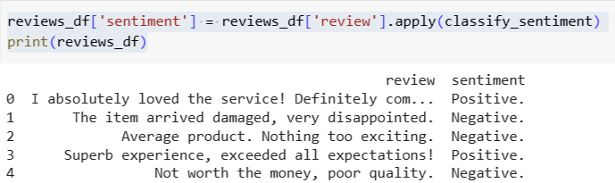
reviews_df['sentiment'] = reviews_df['review'].apply(classify_sentiment)
print(reviews_df)

After defining the reviews, we’ll apply the classify_sentiment function to each review in the DataFrame. This will generate a new column, sentiment, where the IBM Granite model classifies each review as Positive, Negative, or Neutral. By printing the updated reviews_df, we can see the original text and its corresponding sentiment classification.

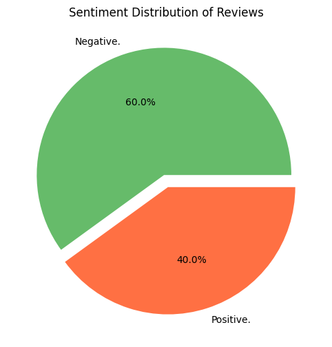
import matplotlib.pyplot as plt


sentiment_counts = reviews_df['sentiment'].value_counts()


plt.figure(figsize=(8, 6))
sentiment_counts.plot.pie(autopct='%1.1f%%', explode=[0.05]*len(sentiment_counts), colors=['#66bb6a', '#ff7043', '#42a5f5'])
plt.ylabel('')
plt.title('Sentiment Distribution of Reviews')
plt.show()

Lastly, we’ll visualize the sentiment distribution in a pie chart. This step provides a clear, intuitive overview of how the reviews are classified, making interpreting the model’s overall performance easier. Matplotlib lets us quickly see the proportion of Positive, Negative, and Neutral sentiments, bringing your sentiment analysis pipeline full circle.

In conclusion, we have successfully implemented a powerful sentiment analysis pipeline using IBM’s Granite 3B open-source model hosted on Hugging Face. You learned how to leverage pre-trained models to quickly classify text into positive, negative, or neutral sentiments, visualize insights effectively, and interpret your findings. This foundational approach allows you to easily adapt these skills to analyze datasets or explore other NLP tasks. IBM’s Granite models combined with Hugging Face Transformers offer an efficient way to perform advanced NLP tasks.

Here is the Colab Notebook. Also, don’t forget to follow us on Twitter and join our Telegram Channel and LinkedIn Group. Don’t Forget to join our 80k+ ML SubReddit.

Recommended Read- LG AI Research Releases NEXUS: An Advanced System Integrating Agent AI System and Data Compliance Standards to Address Legal Concerns in AI Datasets

The post A Coding Guide to Sentiment Analysis of Customer Reviews Using IBM’s Open Source AI Model Granite-3B and Hugging Face Transformers appeared first on MarkTechPost.